
How Convolutional Layers Work in Deep Learning Neural Networks?
An animated ELI5 way to understand convolutions and its parameters

In deep learning, convolutional layers have been major building blocks in many deep neural networks. The design was inspired by the visual cortex, where individual neurons respond to a restricted region of the visual field known as the receptive field. A collection of such fields overlap to cover the entire visible area.
Though convolutional layers were initially applied in computer vision, its shift-invariant characteristics have allowed convolutional layers to be applied in natural language processing, time series, recommender systems, and signal processing.
The easiest way to understand a convolution is by thinking of it as a sliding window function applied to a matrix. This article will see how 1D convolution works and explore the effects of each parameter.
How does convolution work? (Kernel size = 1)
Convolution is a linear operation that involves a multiplicating of weights with input and producing an output. The multiplication is performed between an array of input data and an array of weights, called a kernel (or a filter). The operation applied between the input and the kernel, is a sum of an element-wise dot product. The result of each operation is a single value.
Let us start with the simplest example, using 1D convolution when you have 1D data. Applying a convolution on a 1D array performs the multiplication of the value in the kernel with every value in the input vector.
Assume that the value in our kernel (also known as “weights”) is “2”, we will multiply each element in the input vector by 2, one after another until the end of the input vector, and get our output vector. The size of the output vector is the same as the size of the input.
First, we multiply 1 by the weight, 2, and get “2” for the first element. Then we shift the kernel by 1 step, multiply 2 by the weight, 2 to get “4”. We repeat this until the last element, 6, and multiply 6 by the weight, and we get “12”. This process produces the output vector.
in_x.shape torch.Size([1, 1, 6])
tensor([[[1., 2., 3., 4., 5., 6.]]])
out_y.shape torch.Size([1, 1, 6])
tensor([[[ 2.,  4.,  6.,  8., 10., 12.]]], grad_fn=<SqueezeBackward1>)
Effect of kernel size (Kernel size = 2)
The different sized kernel will detect differently sized features in the input and, in turn, will result in different sized feature maps. Let’s look at another example, where the kernel size is 1x2, with the weights “2”. Like before, we slide the kernel across the input vector over each element. We perform convolution by multiply each element to the kernel and add up the products to get the final output value. We repeat this multiplication and addition, one after another until the end of the input vector, and produce the output vector.
First, we multiply 1 by 2 and get “2”, and multiply 2 by 2 and get “2”. Then we add the two numbers, 2 and 4, and we get “6”–that is the first element in the output vector. We repeat the same process until the end of the input vector and produce the output vector.
in_x.shape torch.Size([1, 1, 6])
tensor([[[1., 2., 3., 4., 5., 6.]]])
out_y.shape torch.Size([1, 1, 5])
tensor([[[ 6., 10., 14., 18., 22.]]], grad_fn=<SqueezeBackward1>)
How to calculate the output vector’s shape
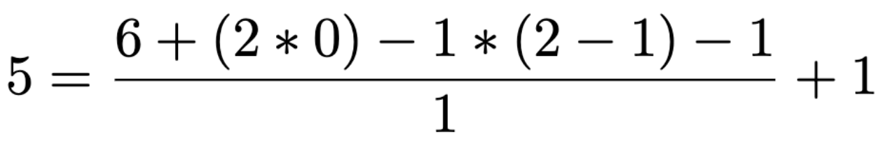
As you might have noticed, the output vector is slightly smaller than before. That is because we increased the kernel’s size, from 1x1 to 1x2. Looking at the PyTorch documentation, we can calculate the output vector’s length with the following:
![Calculate the shape of the output. [https://pytorch.org/docs/stable/generated/torch.nn.Conv1d.html#torch.nn.Conv1d]](/assets/img/posts/how-convolutional-layers-work-deep-learning-neural-networks-09.png)
If we apply a kernel with size 1x2 on an input vector of size 1x6, we can substitute the values accordingly and get the output length of 1x5:
Calculate the output feature’s size is essential if you are building neural network architectures.
Common kernel sizes are in odd numbers (Kernel size = 3)
In the previous example, a kernel size of 2 is a little uncommon, so let’s take another example where our kernel size is 3, where its weights are “2”. Like before, we perform convolution by multiply each element to the kernel and add up the products. We repeat this process until the end of the input vector, which produces the output vector.
Likewise, the output vector is smaller than the input. Applying a 1x3 kernel on a 1x6 input vector will result in a feature vector with a size of 1x4.
In image processing, it is common to use 3×3, 5×5 sized kernels. Sometimes we might use kernels of size 7×7 for larger input images.
in_x.shape torch.Size([1, 1, 6])
tensor([[[1., 2., 3., 4., 5., 6.]]])
out_y.shape torch.Size([1, 1, 4])
tensor([[[12., 18., 24., 30.]]])
How to produce an output vector of the same size? (Padding)
Applying convolution with a 1x3 kernel on a 1x6 input, we got a shorter output vector, 1x4. By default, a kernel starts on the left of the vector. The kernel is then stepped across the input vector one element at a time until the rightmost kernel element is on the last element of the input vector. Thus, the larger the kernel size is, the small the output vector is going to be.
When to use paddings? Sometimes, it is desirable to produce a feature vector of the same length as the input vector. We can achieve that by adding padding. Padding is adding zeros at the beginning and the end of the input vector.
By adding 1 padding to the 1x6 input vector, we are artificially creating an input vector with size 1x8. This adds an element at the beginning and the end of the input vector. Performing convolutions with a kernel size of 3, the output vector is essentially the same size as the input vector. The padding added has zero value; thus it has no effect on the dot product operation when the kernel is applied.
For a convolution with a kernel size of 5, we can also produce an output vector of the same length by adding 2 paddings at the front and the end of the input vector. Likewise, for images, applying a 3x3 kernel to the 128x128 images, we can add a border of one pixel around the outside of the image to produce the size 128x128 output feature map.
in_x.shape torch.Size([1, 1, 6])
tensor([[[1., 2., 3., 4., 5., 6.]]])
out_y.shape torch.Size([1, 1, 6])
tensor([[[ 6., 12., 18., 24., 30., 22.]]])
in_x.shape torch.Size([1, 1, 6])
tensor([[[1., 2., 3., 4., 5., 6.]]])
out_y.shape torch.Size([1, 1, 6])
tensor([[[12., 20., 30., 40., 36., 30.]]])
We can shift the kernel by more steps (Stride)
So far, we have been sliding the kernel by 1 step at a time. The amount of movement on the kernel to the input image is referred to as “stride”, the default stride value is 1. But we can always shift the kernel by any number of elements, by increasing the stride size.
For example, we can shift our kernel with a stride of 3. First, we will multiply and sum the first three elements. Then we will slide the kernel by three steps and perform the same operation for the next three elements. As a result, our output vector is of size 2.
When to increase stride size? In most cases, we increase the stride size to down-sample the input vector. Applying a stride size of 2 will reduce the length of the vector by half. Sometimes, we can use a larger stride to replace pooling layers to reduce the spatial size, reducing the model’s size and increasing speed.
in_x.shape torch.Size([1, 1, 6])
tensor([[[1., 2., 3., 4., 5., 6.]]])
out_y.shape torch.Size([1, 1, 2])
tensor([[[12., 30.]]])
Increase the convolution’s receptive field (Dilation)
While you were reading deep learning literature, you may have noticed the term “dilated convolutions”. Dilated convolutions “inflate” the kernel by inserting spaces between the kernel elements, and a parameter controls the dilation rate. A dilation rate of 2 means there is a space between the kernel elements. Essentially, a convolution kernel with dilation = 1 corresponds to a regular convolution.
Dilated convolutions are used in the DeepLab architecture, and that is how the atrous spatial pyramid pooling (ASPP) works. With ASPP, high-resolution input feature maps were extracted, and it manages to encode image context at multiple scales. I have also applied dilated convolutions in my work for signal processing, as it can effectively increase the output vector’s receptive field without increasing the kernel size (without increasing the model’s size too).
When to use dilated convolutions? Generally, dilated convolutions have shown better segmentation performance in DeepLab and in Multi-Scale Context Aggregation by Dilated Convolutions. You might want to use dilated convolutions if you want an exponential expansion of the receptive field without loss of resolution or coverage. This allows us to have a larger receptive field with the same computation and memory costs while preserving resolution.
in_x.shape torch.Size([1, 1, 6])
tensor([[[1., 2., 3., 4., 5., 6.]]])
out_y.shape torch.Size([1, 1, 2])
tensor([[[18., 24.]]])
Separate the weights (Groups)
By default, the “groups” parameter is set to 1, where all the inputs channels are convolved to all outputs. To use groupwise convolution, we can increase the “groups” value; this will force the training to split the input vector’s channels into different groupings of features.
When groups=2, this is essentially equivalent to having two convolution layers side by side, where each only process half the input channels. Each group then produce half the output channels and then subsequently concatenated to form the final output vector.
in_x.shape torch.Size([1, 2, 6])
tensor([[[ 1.,  2.,  3.,  4.,  5.,  6.],
         [10., 20., 30., 40., 50., 60.]]])
torch.Size([2, 1, 1])
out_y.shape torch.Size([1, 2, 6])
tensor([[[  2.,   4.,   6.,   8.,  10.,  12.],
         [ 40.,  80., 120., 160., 200., 240.]]], grad_fn=<SqueezeBackward1>)
Depthwise convolution. Groups are utilized when we want to perform depthwise convolution, for example, if we want to extract image features on R, G, and B channels separately. When groups == in_channels and out_channels == K * in_channels; this operation is also termed in literature as depthwise convolution.
in_x.shape torch.Size([1, 2, 6])
tensor([[[ 1.,  2.,  3.,  4.,  5.,  6.],
         [10., 20., 30., 40., 50., 60.]]])
torch.Size([4, 1, 1])
out_y.shape torch.Size([1, 4, 6])
tensor([[[  2.,   4.,   6.,   8.,  10.,  12.],
         [  4.,   8.,  12.,  16.,  20.,  24.],
         [ 60., 120., 180., 240., 300., 360.],
         [ 80., 160., 240., 320., 400., 480.]]], grad_fn=<SqueezeBackward1>)
In 2012, grouped convolutions were introduced in the AlexNet paper, where their primary motivation was to allow the network’s training over two GPUs. However, there was an interesting side-effect to this engineering hack, that they learn better representations. Training an AlexNet with and without grouped convolutions have different accuracy and computational efficiency. AlexNet without grouped convolutions is less efficient and is also slightly less accurate.
In my work, I have also applied grouped convolutions to effectively trained a scalable multi-task learning model. I can tweak and scale to any number of tasks by tweaking the “group” parameter.
1x1 convolution
Several papers use 1x1 convolutions, as first investigated by Network in Network. It can be confusing to see 1x1 convolutions, and seems like it does not make sense as it is just pointwise scaling.
However, this is not the case because, for example, in computer vision, we are operating over 3-dimensional volumes; the kernels always extend through the full depth of the input. If the input is 128x128x3, then doing 1x1 convolutions would effectively be doing 3-dimensional dot products since the input depth is 3 channels.
In GoogLeNet, the 1×1 kernel was used for dimensionality reduction and for increasing the dimensionality of feature maps. The 1×1 kernel is also used to increase the number of feature maps after pooling; this artificially creates more feature maps of the downsampled features.
In ResNet, the 1×1 kernel was used as a projection technique to match the number of filters of input to the residual output modules in the design of the residual network.
In TCN, the 1×1 kernel was added to account for discrepant input-output widths, as the input and output could have different widths. 1×1 kernel convolution ensures that the elementwise addition receives tensors of the same shape.