An Introduction to Signals

Signal processing might seem like something impenetrably complicated, even to scientists. Even without fully aware of its underlying presence, signal processing is at the heart of our everyday life. This article will explore what a signal is, how we can generate, and store signals in Numpy for machine learning.

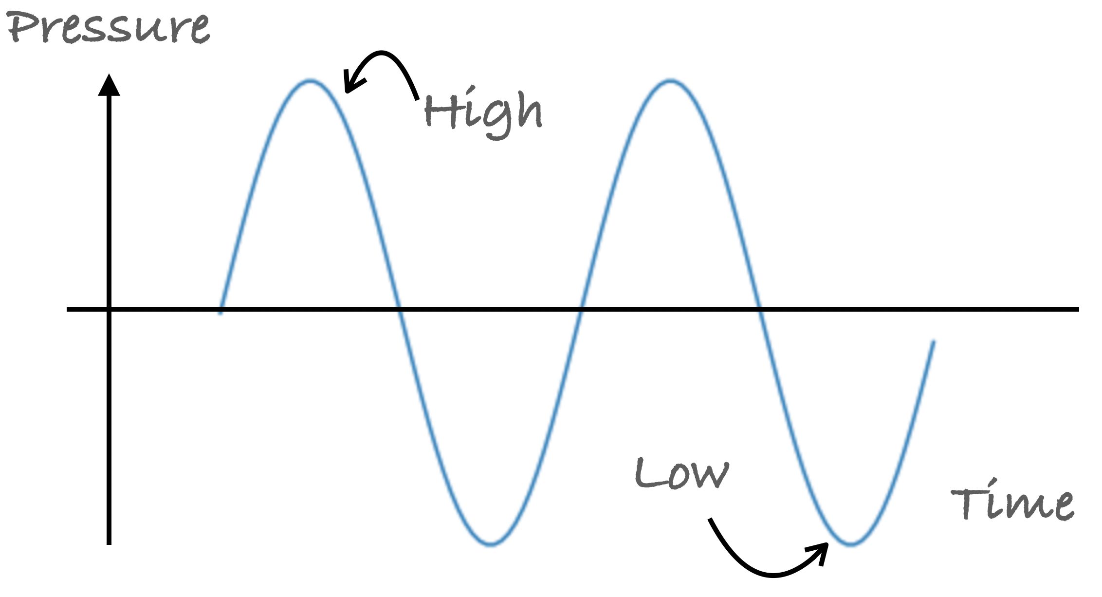
Sound is a wave that results from the back and forth vibration of the medium particles through which the sound wave moves. These sound waves consist of a repeating pattern of high-pressure and low-pressure regions. They are also referred to as pressure waves.

Usually, when we describe sounds, we refer to them in terms of their frequency. We measure these waves by the number of cycles in a second, in a hertz (Hz) measurement unit. The lowest notes your headphones can rumble out are around 20 Hz (in theory!), a 20 Hz note literally refers to the membrane inside the headphone moving to-and-fro 20 times per second. That creates compressed pulses of air which, upon arrival at your eardrum, induces a vibration at the same frequency. Our brain translates these air molecules’ movements that our ears pick up, into something we can recognize. Be it words or music, birds chipping or a car horn.

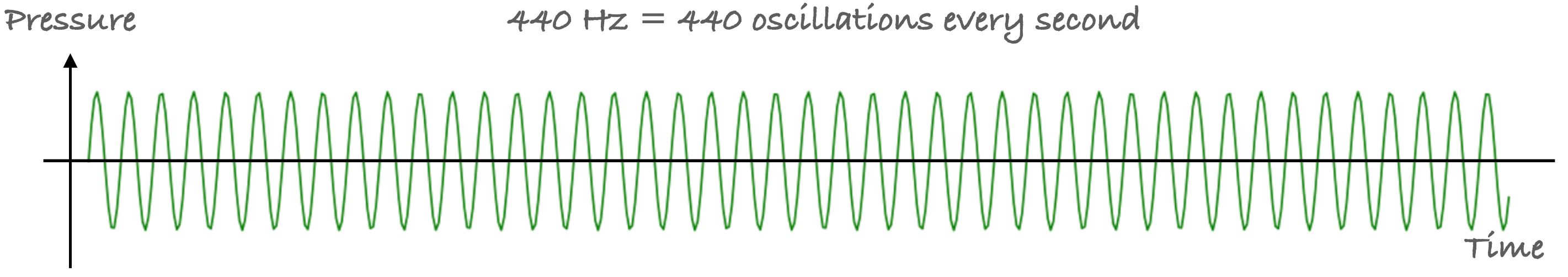
For example, this is a 440 Hz sound wave, the sound of the A note above the middle C on the piano:

440 Hz audio tone by MediaCollege (right click and open in a new tab)

If we were to measure this sound and convert it into a digital signal in a function of time. This is the graph we will get, a 440 Hz sine wave. It oscillates up and down at the equilibrium, at 440 oscillations every second.

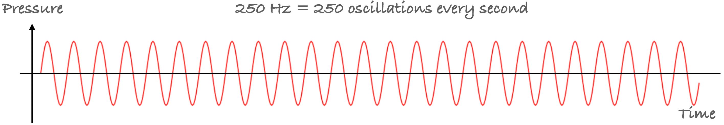
Let’s take another sound wave, 250 Hz, which sounds like this:

250 Hz audio tone by MediaCollege (right click and open in a new tab)

A 250 Hz tone has a lower pitch than 440 Hz. If we were to plot it, It will look similar to the 440 Hz wave but with a lower frequency. It oscillates at 250 oscillations per second.

A single sound wave alone isn’t exciting. But when we combine a few frequencies and play them in the right sequence, we can produce music. We make these sound waves with our vocal cord to speak words that we use for communication.

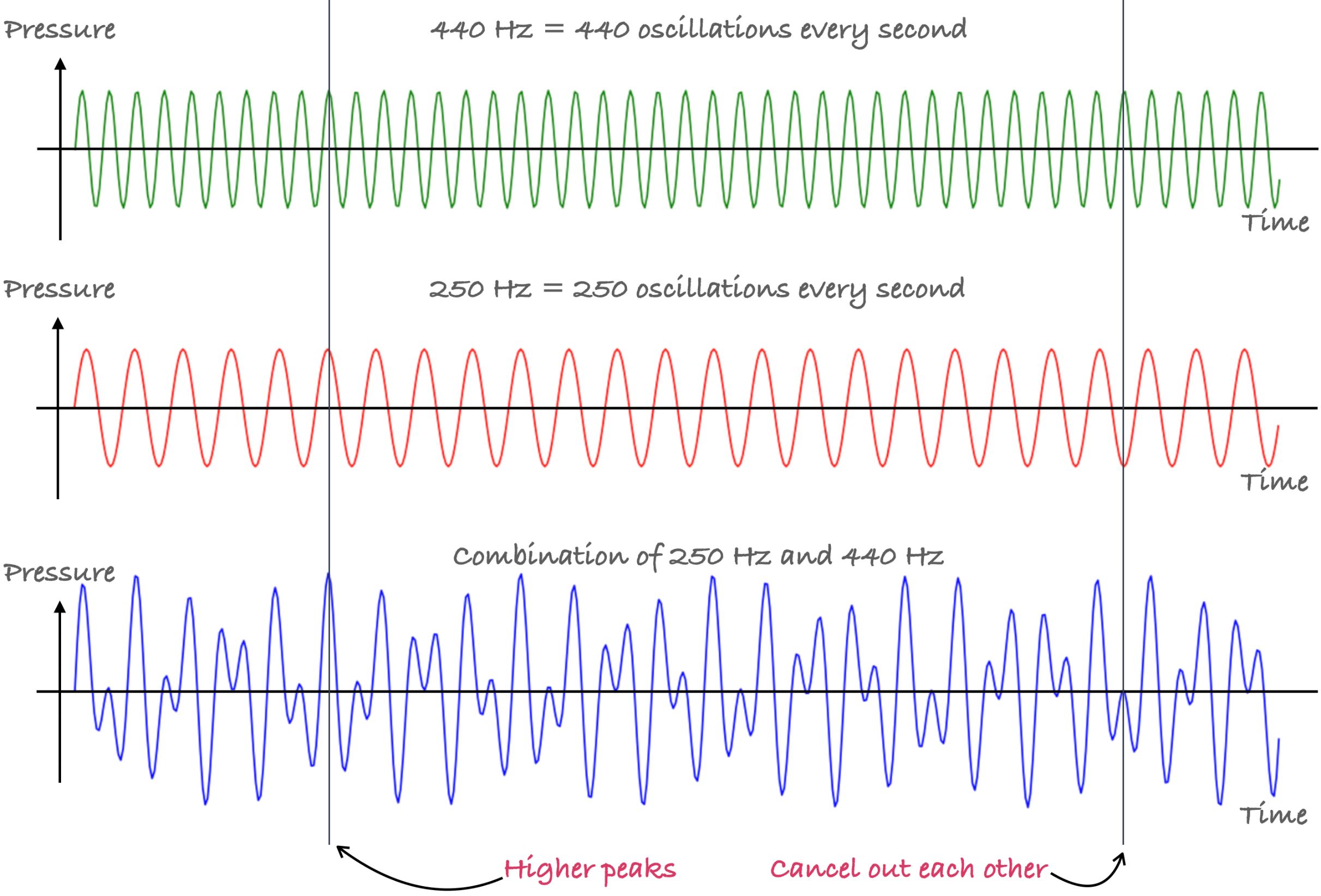
When we combine two frequencies and play them together, the new sound wave is the sum of the two sound waves. What we get is a new wave that is not a pure sine wave. At some points, the peaks add up to become higher, while other points cancel out each other resulting in zero.

We can add more sound frequencies; the sound wave will get more and more complicated. In fact, these complicated sound waves are what our microphones pick up. Our microphones pick up many different frequencies at any point in time; the final recordings are the sum of all the sound frequencies combined. Other than those sound that you actually want to record, it also picks up background noise, echos, and even some electric signal noise.

Even though these examples are on sound waves, these concepts are also applied in other digital signals such as an electrocardiogram and electroencephalogram.

So how do we store signals digitally?

As analog signals are continuous in both time and amplitude, we need to reduce the signal into a discrete-time signal, both in time and amplitude. This signal reduction process is call sampling. The sampling rate defines the number of data points in one second, literally how fast samples are taken.

The sampling rate determines the signal’s fidelity. There is a minimum sampling rate for each signal to preserve the information contained in the signal. According to the Nyquist–Shannon sampling theorem, the sampling rate must be at least twice the signal’s maximum frequency to allow the signal to be completely represented. This means that if the signal contains high-frequency components, we will need to sample at a higher rate.

In theory, as long as the Nyquist limit, which is half the sample rate, exceeds the highest frequency of the signal being sampled, the original analog signal can be reconstructed without loss. Otherwise, the signal information may not be completely represented, where some of the original signal frequencies may be lost. It will result in audible artifacts known as “aliasing,” which are unwanted components in the reconstructed signal.

Let’s take a look at what happens when the sampling rate gets too low.

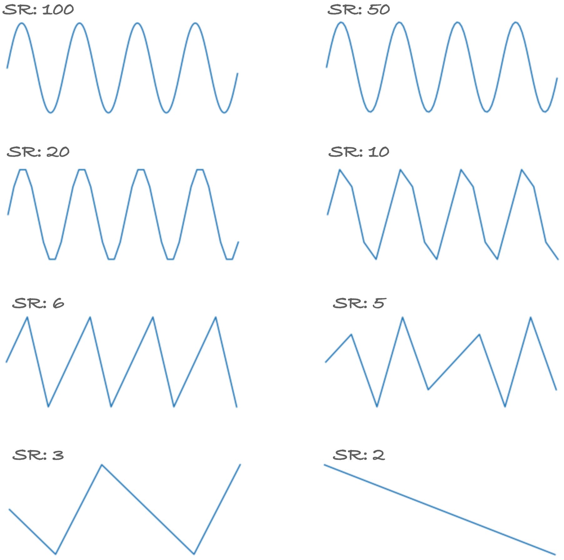
The figure above shows a 2 Hz signal lasting 2-seconds; it has four oscillations in total, two oscillations per second. At a sampling rate of 50 and 100, the wave looks excellent as there are enough data points. We start to see edges in the signal at 10 and 20 sampling rates though we can still clearly see four positive peaks. The signal begins to lose some information when the sampling rate falls below 6.

As humans can hear 20–20,000 Hz range; this is why audio waveform and early professional audio equipment manufacturers chose sampling rates at 44.1kHz, the “standard” sampling rate for many digital formats. Increasing the sampling rate generally improves the sound quality, but it also increases the disk space required to store. Many telephone and walkie-talkie signals are transmitted on 8,000 Hz to reduce packet size to improve transmission.

For machine learning, sampling at higher frequencies results in better-reconstructed signals, resulting in better performance. However, this requires faster CPU/GPU to convert and process the signals, and a bigger GPU memory is needed as it also increases the model’s size as your inputs get larger. Therefore, we must weigh each application’s advantages and disadvantages and be aware of the tradeoffs involved.

So far, we have seen signals with a single channel. But signals in real-world applications can have multiple channels. For example, we have two channels in audio, left and right channels. In electroencephalography and electrocardiography, we can have ten or more channels. Neuralink aims to build an integrated brain-machine interface platform with thousands of channels.

Generate some signals (in Python)

We can generate signals with three parameters, 1) signal duration, sampling rate, and frequencies.

As we are storing the signals as a sequence of numbers, first, we need the number of data points of the signal. This can be done by multiplying the signal duration with the sampling rate. Next, we need a time variable, a function over time that allows us to generate the waveform for each data point.

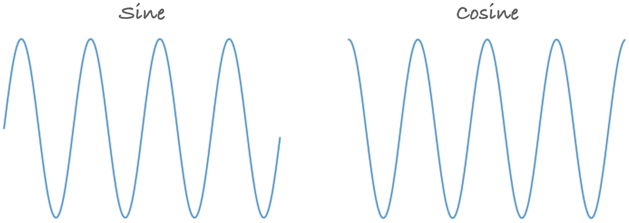
We can either generate a sine or a cosine wave with a sine/cosine periodic function. The sine function tracks the y-coordinates of a point traveling around the unit circle while the cosine function follows the x-coordinates.

Using either function will generate a similar but different wave.

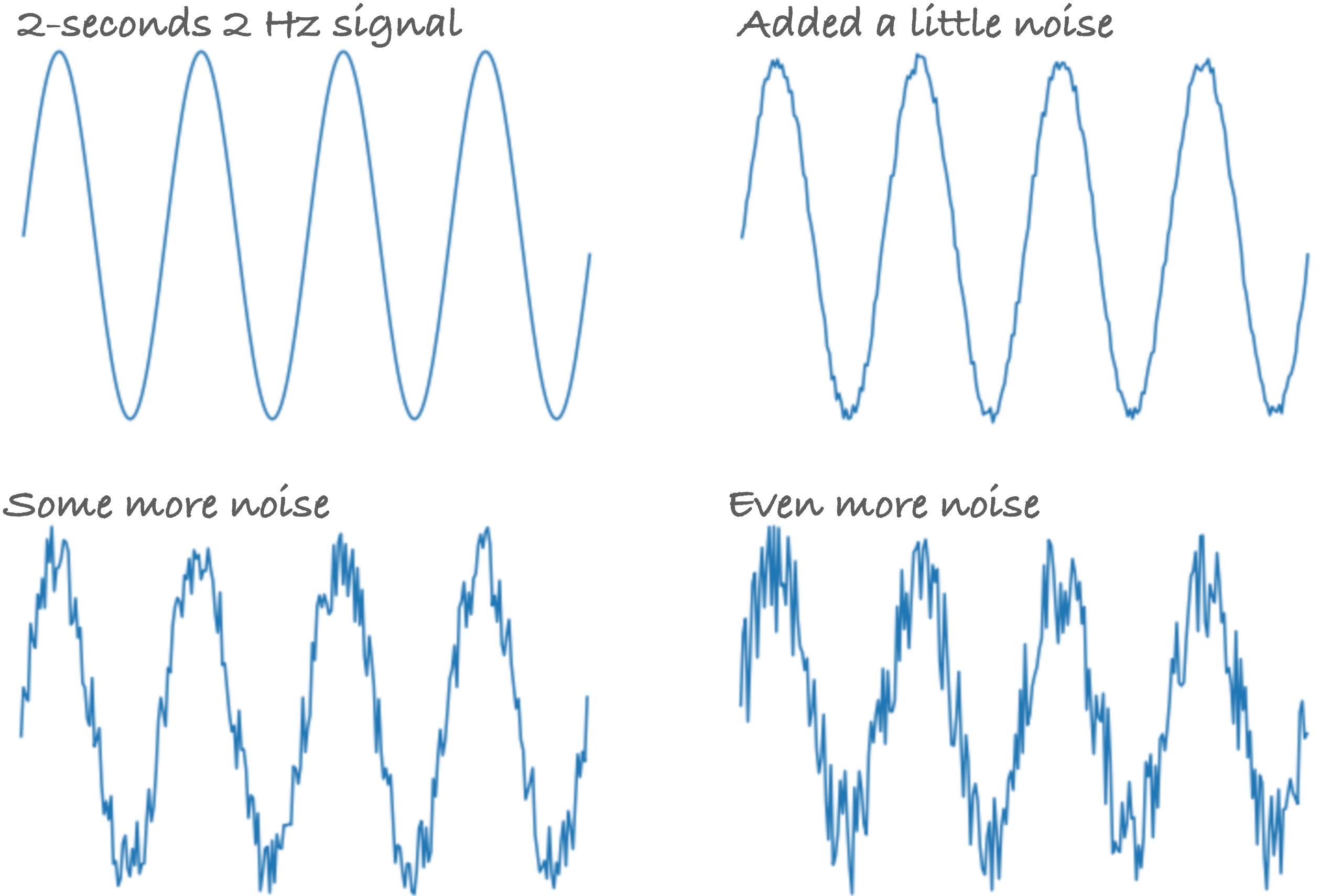
To create a more realistic signal, we can also add noise to the generated signal by adding random values to each data point. This allows us to test our model ability to generalize and learn from a noisy dataset.

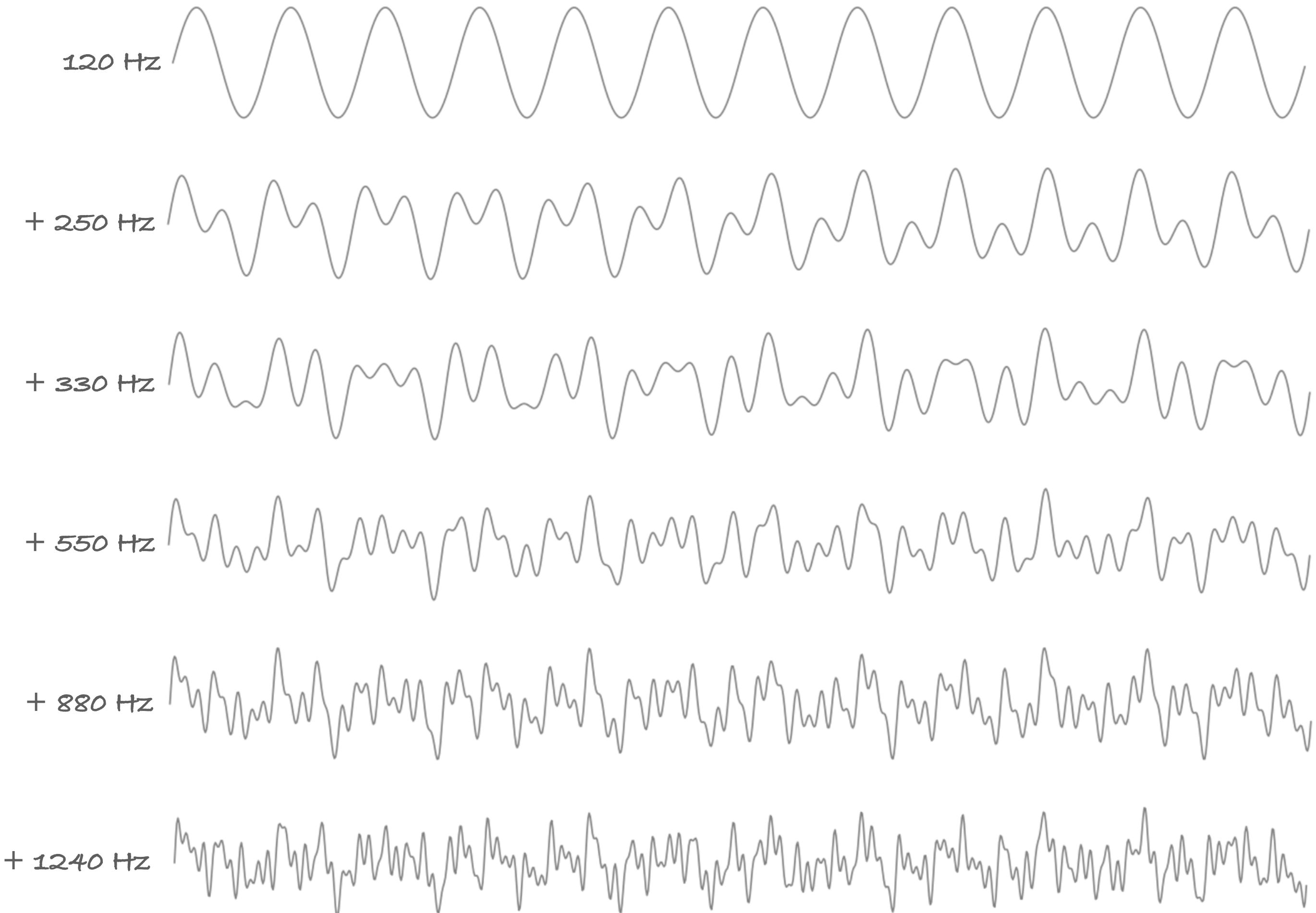
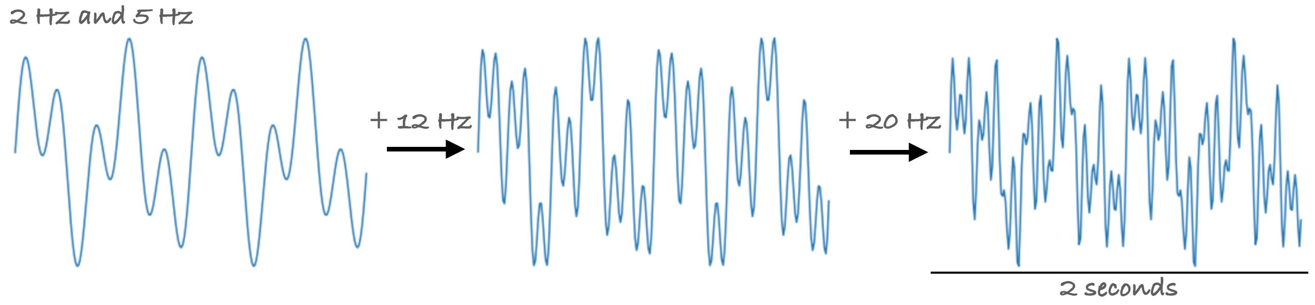
Recapping from the previous sections, the value of a point is the sum of all the frequencies. If we want to generate a signal that contains more than one frequencies, we can simply sum each generated waveform. Here are some examples of generated signals; each wave adds additional frequencies to the previous:

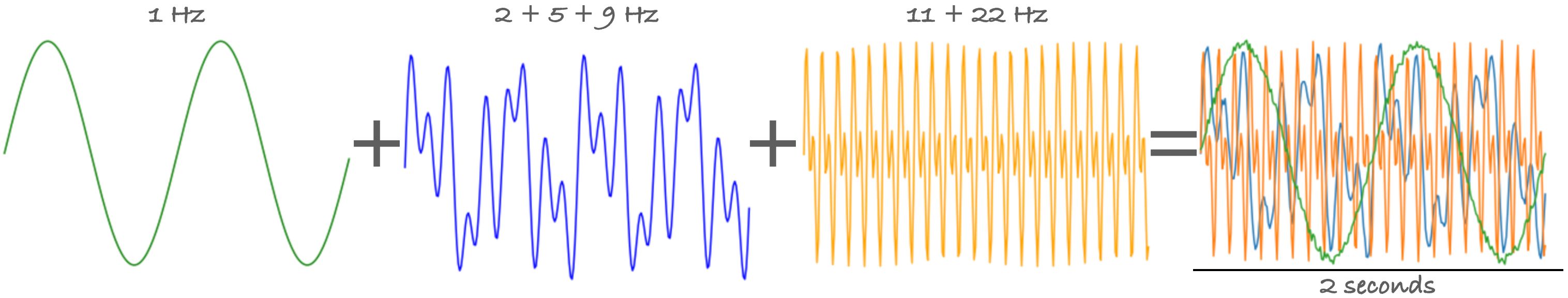
Lastly, an example of a multiple channel signal:

Here are the codes from the torchsignal package if you plan to generate some signals.

With this code, you could generate your own datasets, where the input features are the raw signals (with noise), and the predicted outputs are the frequencies.

As I am currently working on my Ph.D. on brain-computer interface research, I’ve made a repo containing codes commonly used in signal processing. This package includes functions to clean signals and other signal processing techniques. Feel free to check it out and star this repo, torchsignal.

Seeking for collaborators to contribute new features, utility functions, bug fixes, and documentation. Currently, I am working on this alone. If you are working on signal processing or brain-computer interface, and keen to build a high-quality package to apply PyTorch to the signal processing domain, do reach out to me.

Generating signals is useful for creating ideal datasets to test models’ performance in a “lab environment.” In the next article, I will introduce how we can filter and clean signals for machine learning models.