
Time Series Forecasting with TensorFlow.js
Pull stock prices from online API and perform predictions using Recurrent Neural Network & Long Short Term Memory (LSTM) with TensorFlow.js framework
Machine learning is becoming increasingly popular these days and a growing number of the world’s population see it is as a magic crystal ball: predicting when and what will happen in the future. This experiment uses artificial neural networks to reveal stock market trends and demonstrates the ability of time series forecasting to predict future stock prices based on past historical data.
Disclaimer: As stock markets fluctuation are dynamic and unpredictable owing to multiple factors, this experiment is 100% educational and by no means a trading prediction tool.
| Explore Demo |
| View Code |
Project Walkthrough
There are 4 parts to this project walkthrough:
- Get stocks data from online API
- Compute simple moving average for a given time window
- Train LSTM neural network
- Predict and compare predicted values to the actual values
Get Stocks Data
Before we can train the neural network and make any predictions, we will first require data. The type of data we are looking for is time series: a sequence of numbers in chronological order. A good place to fetch these data is the Alpha Vantage Stock API. This API allows us to retrieve chronological data on specific company stocks prices from the last 20 years. You may also refer to this article that explains adjusted stock prices, which is an important technical concept for working with historical market data.
The API yields the following fields:
- open price
- the highest price of that day
- the lowest price of that day
- closing price (this is used in this project)
- volume
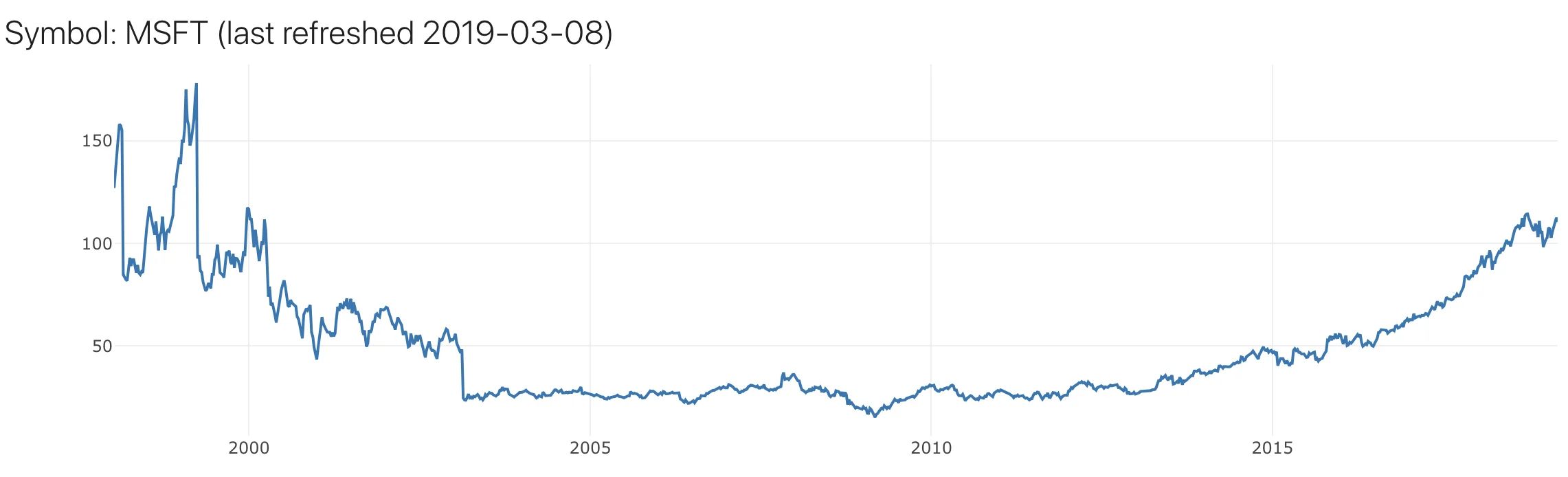
To prepare training dataset for our neural network, we will be using closing stocks price. This also means that we will be aiming to predict the future closing price. Below graph shows 20 years of Microsoft Corporation weekly closing prices.
Simple Moving Average
For this experiment, we are using supervised learning, which means feeding data to the neural network and it learns by mapping input data to the output label. One way to prepare the training dataset is to extract the moving average from that time-series data.
Simple Moving Average (SMA) is a method to identify trends direction for a certain period of time, by looking at the average of all the values within that time window. The number of prices in a time window is selected experimentally.
For example, let’s assume the closing prices for the past 5 days were 13, 15, 14, 16, 17, the SMA would be (13+15+14+16+17)/5 = 15. So the input for our training dataset is the set of prices within a single time window, and its label is the computed moving average of those prices.
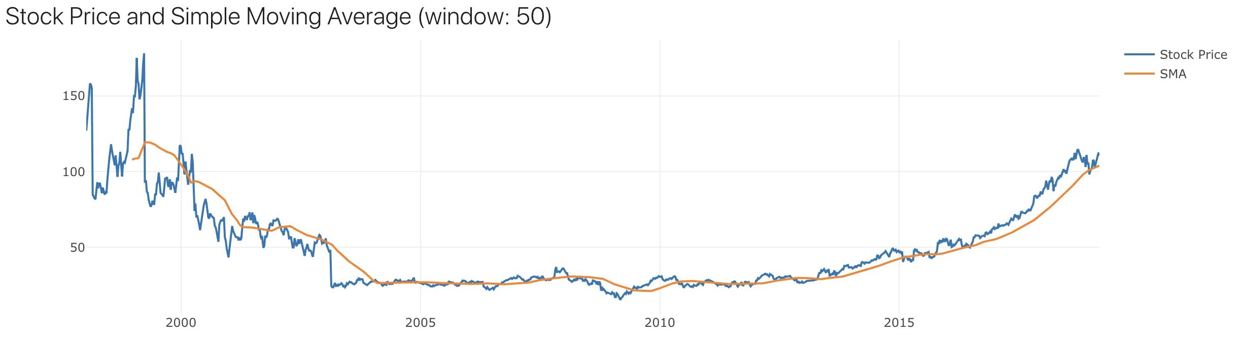
Let’s compute the SMA of Microsoft Corporation weekly closing prices data, with a window size of 50.
function ComputeSMA(data, window_size)
{
  let r_avgs = [], avg_prev = 0;
  for (let i = 0; i <= data.length - window_size; i++){
    let curr_avg = 0.00, t = i + window_size;
    for (let k = i; k < t && k <= data.length; k++){
      curr_avg += data[k]['price'] / window_size;
    }
    r_avgs.push({ set: data.slice(i, i + window_size), avg: curr_avg });
    avg_prev = curr_avg;
  }
  return r_avgs;
}
And this is what we get, weekly stock closing price in blue, and SMA in orange. Because SMA is the moving average of 50 weeks, it is smoother than the weekly price, which can fluctuate.
Training Data
We can prepare the training data with weekly stock prices and the computed SMA. Given the window size is 50, this means that we will use the closing price of every 50 consecutive weeks as our training features (X), and the SMA of those 50 weeks as our training label (Y). Which looks like that…
Next, we split our data into 2 sets, training and validation set. If 70% of the data is used for training, then 30% for validation. The API returns us approximate 1000 weeks of data, so 700 for training, and 300 for validation.
Train Neural Network
Now that the training data is ready, it is time to create a model for time series prediction, to achieve this we will use TensorFlow.js framework. TensorFlow.js is a library for developing and training machine learning models in JavaScript, and we can deploy these machine learning capabilities in a web browser.
Sequential model is selected which simply connects each layer and pass the data from input to the output during the training process. In order for the model to learn time series data which are sequential, recurrent neural network (RNN) layer is created and a number of LSTM cells are added to the RNN.
The model will be trained using Adam (research paper), a popular optimisation algorithm for machine learning. Root mean square error which will determine the difference between predicted values and the actual values, so the model is able to learn by minimising the error during the training process.
Here is a code snippet of the model described above, full code on Github.
These are the hyper-parameters (parameters used in the training process) available for tweaking in the frontend:
- Training Dataset Size (%): the amount of data used for training, and remaining data will be used for validation
- Epochs: number of times the dataset is used to train the model (learn more)
- Learning Rate: the amount of change in the weights during training in each step (learn more)
-
Hidden LSTM Layers: to increase the model complexity to learn in higher dimensional space (learn more)
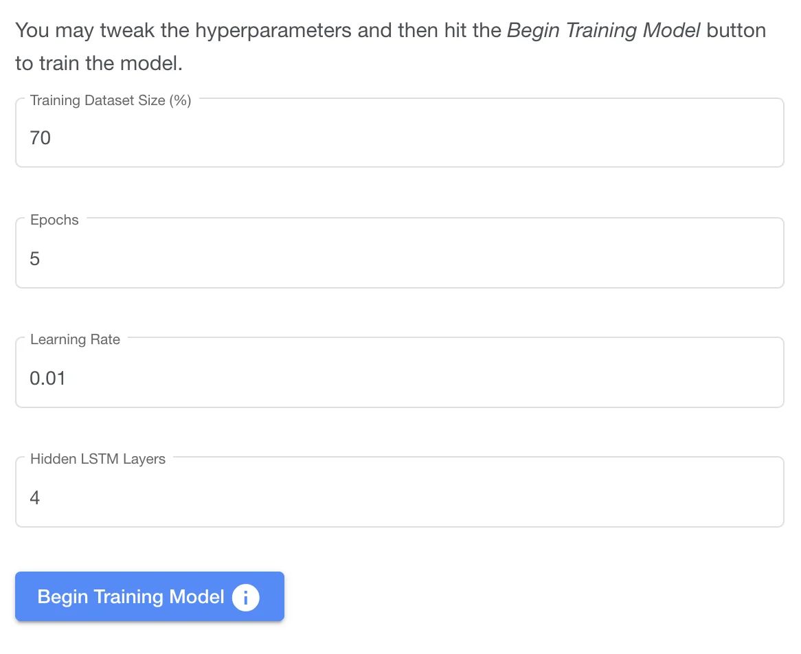
Click the Begin Training Model button…
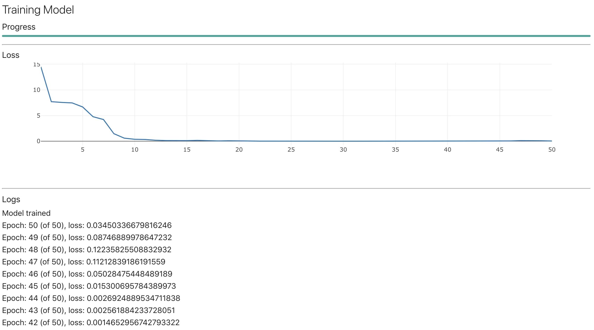
The model seems to converge at around 15 epoch.
Validation
Now that the model is trained, it is time to use it for predicting future values, for our case, it is the moving average. We will use the model.predict function from TFJS.
The data has been split into 2 sets, training and validation set. The training set has been used for training the model, thus will be using the validation set to validate the model. Since the model has not seen the validation dataset, it will be good if the model is able to predict values that are close to the true values.
So let us use the remaining data for prediction which allow us to see how closely our predicted values are compared to the actual values.
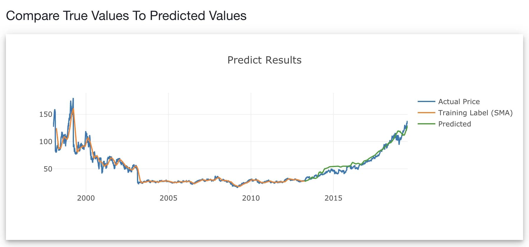
Looks like the model predicted (green line) does a good job plotting closely to the actual price (blue line). This means that the model is able to predict the last 30% of the data which was unseen by the model.
Other algorithms can be applied and uses the Root Mean Square Error to compare 2 or more models performance.
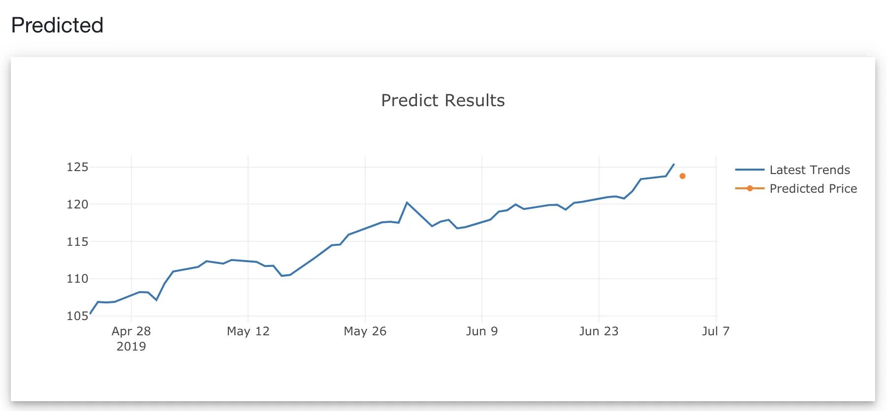
Prediction
Finally, the model has been validated and the predicted values map closely to its true values, we shall use it to predict the future. We will apply the same model.predict function and use the last 50 data points as the input, because our window size is 50. Since our training data is increment daily, we will use the past 50 days as input, to predict the 51st day.
Why Isn’t My Model Performing?
The model has never seen similar data in the past. In March 2020, where the market dipped and recovered within a month or two, this has never happened in history. The model is likely to fail to predict drastic changes in stock prices during those periods.
We can add more features. In a general sense, more features tend to make the model perform better. We can include trading indicators such as Moving average convergence divergence (MACD), Relative strength index (RSI), or Bollinger bands.
Add even more features. Another amazing API that Alpha Vantage API provides is Fundamental Data. This means that you can also include annual and quarterly income statements and cash flows for the company of interest. Who knows, those features might be useful.
There could have many other reasons why the model fails to learn and predict. This is the challenge of machine learning; it is both an art and science to build good performing models.
Conclusion
There are many ways to do time series prediction other than using a simple moving average. Possible future work is to implement this with more data from various sources.
With TensorFlow.js, machine learning on a web browser is possible, and it is actually pretty cool.
Explore the demo on Github, this experiment is 100% educational and by no means a trading prediction tool.